Dynamic Programming Memoization with Trees

Recently I came by the House Robber III problem in LeetCode. The basic idea in this problem is you’re given a binary tree with weights on its vertices and asked to find an independent set that maximizes the sum of its weights. This is a dynamic programming problem rated medium in difficulty by the website.

This post starts with a brief overview on dynamic programming, and ends with an anecdote on how I tried two different implementations of dynamic programming memoization when solving the House Robber III problem. Although the actual algorithmic idea in both approaches is the same, the strategy used to store memozation matrices when entries are the nodes of a tree led to considerable differences in readability.

Dynamic Programming

Dynamic programming is an algorithm design technique in which a problem is solved by combining stored solutions of smaller subproblems. The idea is that by storing solutions to smaller problems and systematically referring to them later you can search through all possible solutions without having to repeat computations. In this sense there commonly exists – although not necessarily – a time-space tradeoff when implementing a dynamic programming algorithm. A gain in time can be achieved by referring to precomputed solutions instead of repeating yourself, while paying with more space to store said solutions.

For more explanation about dynamic programming and other algorithm design techniques I recommend the book The Algorithm Design Manual by Prof. Steven S. Skiena.

The simplest example of the technique, though it isn’t always framed as a dynamic programming problem, is probably the problem of finding the $n$-th member of the Fibonacci sequence defined by $F_n = F_{n-1} + F_{n-2}$, with $F_0 = 0$ and $F_1 = 1$. The definition of this problem itself can already be used as a dynamic programming memoization matrix. The traditional naive recursive solution in C++ is

int fibonacci(int n) {
    if (n == 0 || n == 1) return n;
    return fibonacci(n - 1) + fibonacci(n - 2);
}

This solution spawns two new recursive function calls in every iteration, generating a call tree of height $n$. Such a pattern characterizes an $O(2^n)$ complexity algorithm. An exponential algorithm for such a simple problem is pretty bad.

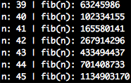
I can answer this faster than my computer

I was patient enough to run this algorithm in my machine up to input $n=45$, at which point execution was so slow I could answer for $n=46$ faster than my computer by adding up the two last answers with a calculator. This is the exact realization that enables dynamic programming to be applied in this problem. By memorizing previous answers and systematically accessing them later we can get rid of the two recursive function calls altogether. That would grant us an $O(n)$ solution. Much better.

Let’s start off this new approach by defining our memoization matrix. Suppose we have an array $D_{0..n}$ of size $n+1$, where its $k$-th entry, denoted $D_k$, corresponds to the $k$-th member of the Fibonacci sequence. Provided such an array, it’s easy to see we can find the $n$-th member simply by computing $D_{n-1} + D_{n-2}$. From the base cases of the problem we know $D_0 = 0$ and $D_1 = 1$. Now notice how the solution of a subproblem $D_k$ requires that the previous subproblems $D_{k-1}$ and $D_{k-2}$ have already been solved. This constraint can be satisfied by iteratively finding the subsolutions from $D_2$ up to $D_{k-1}$. This way whenever we need a previous solution we can be sure it has been computed beforehand and its solution stored in $D$. By the end of this process the $n$-th member of the Fibonacci sequence will be stored in $D_k$.

int fibonacci(int n) {
    if (n == 0 || n == 1) return n;
    // alocate our memorization array
    int memory[n + 1];
    // initialize with base cases
    memory[0] = 0; memory[1] = 1;
    // solve all smaller sub problems until getting to our goal
    for (int i = 2; i <= n; ++i)
        memory[i] = memory[i - 1] + memory[i - 2];
    return memory[n];
}

This implementation runs instantaneously for values of $n$ way past what a C++ 64-bit long long int would represent. Notice this algorithm now requires $O(n)$ additional space for the memory array. These bounds can be further improved to constant space while maintaining $O(n)$ time by realizing that only the last two entries of the memoization array are needed to solve a subproblem.

As stated earlier, although the $n$-th member of the Fibonacci sequence is among the simplest dynamic programming examples one can find, it serves well for our purposes here. The discussion above illustrates how the idea of systematically storing answers in a memoization matrix can help you speed up algorithm execution by solving a problem with table lookups instead of recomputation.

Now we’re on the same page with respect to the dynamic programming technique, let’s have a deeper look into the House Robber III problem and independent sets in trees.

Maximum-Weight Independent Sets in Trees

$\newcommand{\dbar}[0]{\overline{D}}$ In this problem we are asked to find an independent set that maximizes the sum of the weights of its vertices. Given a graph $G=(V,E)$, an independent set of $G$ is defined mathematically as a subset $S$ of $V$ such that for any edge $(u,v) \in E$, either $u \notin S$ or $v \notin S$. More simply put, an independent set of a graph is a subset of its vertices in which no two vertices are adjacent. The problem of finding the maximum-weight independent set is actually known to be $NP$-Hard for general graphs. However, in House Robber III we happen to be dealing strictly with trees. For this subclass of graphs we shall see that a polynomial algorithm does exists.

We start solving the problem with dynamic programming by defining the memoization array. Assuming $n$ is the number of nodes in the tree, suppose we have two arrays $D$ and $\dbar$, each of size $n$, where the $k$-th entry of $D$ ($\dbar$), denoted $D_k$ ($\dbar_k$), corresponds to the total weight of the maximum-weight independet set of the subtree rooted at the $k$-th node that includes (excludes) the $k$-th node. After the arrays $D$ and $\dbar$ have been entirely computed, the answer of the problem will correspond to the maximum among $D_r$ and $\dbar_r$, where $r$ is the node that represent the root of the tree.

The base case of this dynamic programming solution are the leaves of the tree. Given a leaf node $l$ we have that $D_l = w_l$ and $\dbar_l = 0$, where $w_l$ is the weight of the $l$-th node.

At the general case we wish to solve the maximum-weight independent set of the subtree rooted at the $k$-th node. Both $D_k$ and $\dbar_k$ can be computed in constant time. The solution $D_k$ has to contain the $k$-th node, thus, by the definition of independent sets, it can’t contain either of his children. With $\dbar_l$ and $\dbar_r$, where $l$ and $r$ are respectively the left and right children of the $k$-th node, we can know the maximum-weight independent sets on the children of $k$ that do not include them. Hence, $D_k$ corresponds to the addition $w_k + \dbar_l + \dbar_r$. Mathematically we can define $D_k$ as

Similarly, $\dbar_k$ does not contain the $k$-th node, thus, it may or may not contain its children. Both options are allowed so we choose whichever is larger, which means $\dbar_k$ corresponds to the computation of $\max(D_l,\dbar_l) + \max(D_r, \dbar_r)$. More succinctly

From the definitions of $D$ and $\dbar$ we see that solving the subproblem for $k$ requires that the subproblems for its children $l$ and $r$ have already been solved. This constraint can be satisfied by finding subsolutions from the leaves up to the root, which can be fulfilled in either depth-first or breadth-first traversal of the tree.

Let’s have a look at an example to illustrate the idea.

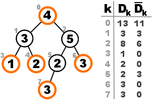
In this tree the outlined independent set has total weight 13, as computed from the complete memoization matrix.

We see that the base case of the memoization arrays are respected in the leaf nodes 3, 4, 6, and 7, where $D_k = w_k$ and $\dbar_k = 0$. Let’s focus our attention at the subtree rooted at node 2 for a moment. We know $D_2$ will be $w_2 = 5$ plus the solutions of its children that do not contain its children. For the left subtree that solution would be $3$, coming from node 7, while from the right subtree that would be $0$, since node 6 has no children.The total solution for node 2 is $D_2 = 5 + 3 + 0 = 8$. On the other hand $\dbar_2$ is the sum of the maximum of the solutions of its children. That means $\dbar_2 = \dbar_5 + D_3$, which corresponds to $3 + 3 = 6$.

This solution requires us to store two arrays of size $n$ each, corresponding to $O(n)$ words of extra memory space. Computing one entry of the arrays is accomplished with no more than a few integer summations and array accesses, which can be done in $O(1)$ time. Overall there are $2n$ entries to be computed, and the algorithm takes $O(n)$ time to solve the maximum-weight independent set problem on trees.

In the following section we explore implementation details of the algorithm defined above.

Memoization Storage in Trees

The input given to our program in LeetCode is the root of a binary tree as typically defined by the TreeNode C++ struct. The rob function is what we have to implement, a function that returns the weight of its maximum-weight independent set.

struct TreeNode {
    int val;
    TreeNode *left, *right;
};

int rob(TreeNode* root);

Looking back at the solution scheme described in the previous section we quickly notice that in order to implement it the traditional dynamic programming way we will need to:

• Find $n$, the size of the tree, so that the $D$ and $\dbar$ memoization arrays can be allocated. The tree structure provides no resort for us to know its size, so this requires a full tree traversal.
• Create a mapping of tree nodes to integers in the interval $[0, n)$, so we know which entry of the memoization arrays correspond to a given node. This can be done along the traversal in the previous requirement by numbering nodes in order of discovery.

Only after these two steps are done we would be able to compute the memoization arrays systematically up to the tree root and solve the problem. This was my first strategy when designing an algorithm. Each of the additional steps require $O(n)$ time, which won’t increase the overall complexity of the solution. Though I went on to implement this approach, and it did work, all along the way I felt like there was more going on with my program than was actually necessary. In case you’re interested this first implementation can be found in this gist.

My problem, and the reason I decided to write this post, was that trees on a pointer implementation tend not to work well with the traditional dinamic programming memoization based on arrays. How can we make this less complex? Or, do we absolutely need arrays at all? With some thought and intuition I quickly realized that the algorithm scheme showed in the previous section could be improved by making use of the tree structure as the memoization matrix storage. This way memoization matrix access is done implicitly, as opposed to an explicit array.

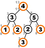
Improved memoization by storing subsolutions in a payload. The number above a node is its $D_k$, while $\dbar_k$ is the number below.

Essentially the concept of the solution algorithm here is the same scheme as the one from last section, except that now the information from the memoization arrays $D$ and $\dbar$ is stored in the tree alongside the node it corresponds to. The final implementation of the improved scheme is shown below.

In this implementation neither there are arrays to be allocated, nor must we create a mapping of nodes to integers. By storing memoization as a payload alongside tree nodes, actual computation related to the problem solution can begin right away. Besides, this led to a more elegant, and more readable solution in half the number of lines.

From now on I will keep in mind that the concept of dynamic programming memoization matrices don’t necessarily have to be implemented as actual matrices. Characteristics of the underlying data structure being applied at the problem in hand can be leveraged to represent the whiteboard abstractions drafted when designing an algorithm.